Conjugate Gradients

This is the fourth post in our series on Krylov subspaces. The previous ones (i.e Arnoldi Iterations and Lanczos Algorithm were mostly focused on eigenvalue and eigenvector computations. In this post we will have a look at solving strategies for linear systems of equations. In particular, we will derive the famous conjugate gradients algorithm.

The conjugate gradients method is one of the most popular solvers for linear systems of equations. There exist countless variations and extensions. You can find a rather broad overview in [1]. The original algorithm can be found in [2]. Variations are for example presented in [3,4,5]. The conjugate gradients method is a Krylov subspace method. It iteratively works on a certain Krylov subspace and will eventually stop after a finite number of iterations with an exact solution (under the assumption that no rounding errors and other artefacts of floating point operations exist).

Problem Derivation

A common problem in applied mathematics is solving linear systems of equations. They appear in all imaginable shapes. Usually you are given a matrix $A$ and a vector $b$ and you would like to find a vector $x$ such that $Ax=b$, or $Ax-b=0$. We would like to approach this task from an optimization point of view. The most popular strategy in mathematical optimization is probably the minimization of some energy. If your energy is a sufficiently smooth function then its minima and maxima are among the set of points for which its first derivative is 0. Assuming we wanted to solve $Ax-b=0$ by such an optimization strategy, we need to find an energy whose first order derivative is given by $Ax-b$.

If $A$, $x$, and $b$ were scalars, then we could integrate $Ax-b$ and obtain the energy $\frac{1}{2}Ax^2-bx$. This gives us a hint, but we have to ensure that dimensions fit. For the moment we have the following restrictions:

1. $A$ is a matrix in $\mathbb{R}^{m,n}$

2. $x$ is a vector in $\mathbb{R}^n$

3. $b$ is a vector in $\mathbb{R}^m$

4. Our energy $E$ should map $\mathbb{R}^n$ to $\mathbb{R}$.

There are two ways to extend the scalar variant $bx$ to vector valued inputs. Either we do a component wise product (i.e. a Hadamard product) or we use a scalar product. A Hadamard product would not lead to a scalar valued energy, hence we should use a scalar product. But then we must also require $n=m$.

Similarly, the only combination of $A$ and $x$ that works with requirements is given by $x^\top A x$. All in all we get the energy

And indeed the gradient of $E$ is given by $\nabla E(x)=Ax-b$. Note that we silently assumed $A$ to be symmetric here. Otherwise, the gradient would be $\frac{1}{2}(A+A^\top) x - b^\top x$.

Our energy should also be "well-behaved". In mathematical terms this usually means that it should have a single minimum and be convex. One way to ensure this is to require $A$ to be positive definite.

Stiefels presentation in [2] is similar. However he also remarks that many tasks, especially in physics, come with some kind of energy formulation. In that case it is recommended to start immediately with the energy and derive the necessary and sufficient optimality conditions directly from the energy. This leads surprisingly often to a linear system of equations.

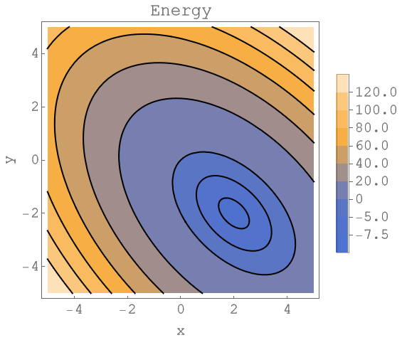
The picture below represents the contour plot of the following linear system of equations

The black ellipses in the plot are the level lines. Along these curves the energy takes a constant value. The solution of this system is $x=2$ and $y=-2$. The energy takes the value $-8$ at this point. We will reuse this example in the following sections.

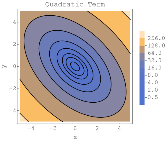
The next plot shows the level lines of the quadratic term $x^\top A x$. Note that the level lines again form ellipses. The term $b^\top x$ only shifts the energy around. The major and minor axis of this ellipse are given by the eigenvectors of the matrix $A$.

An Optimization Strategy

Let's start simple and play a bit with the data at hand. Assume we are at some point $x_0$ and we are given a direction $v$ along which we want to minimize our energy $E$. This means we want to solve

This is optimization task in one dimension with a single unknown. A straightforward expansion of the cost function reveals that $\lambda$ is optimal if

holds. Here $\langle\cdot,\cdot\rangle$ denotes the standard euclidean dot product. We deduce that for optimal $\lambda$, the next residual of our linear system (i.e. $A(x_0 + \lambda v) - b$) will be orthogonal to our current search direction. From this it's easy to see that the optimal step size $\lambda$ is given by

Note that the denominator is always non-zero if $v$ is not the zero vector because we required $A$ to be positive definite. Another interesting observation (albeit a not really surprising one) is that $\lambda=0$ will be the only valid choice when $x_0$ is the solution of your linear system. This could end up as being a nice stopping criteria for our algorithm!

The previous optimization gives us a first hint at how one could minimize $E$: We start somewhere at $x_0$, chose a direction $v$ and run along that direction to minimize $E$. Then we get a new point, chose a new direction and repeat the whole process. As for the direction $v$, it would suffice to chose a direction along which $E$ can be decreased. This direction can either be found by some searching algorithm or if you have some experience with multivariate calculus, then you know that the negative gradient points in direction of the steepest descent. In general, finding descent directions is not that hard. Finding the good ones is challenging, though.

The following plots shows what happens when you simply select two different directions and alternate between minimising the energy along these directions. The yellow line depicts that path of our iterates. The position of the iterates is always at the corner points where we change direction.

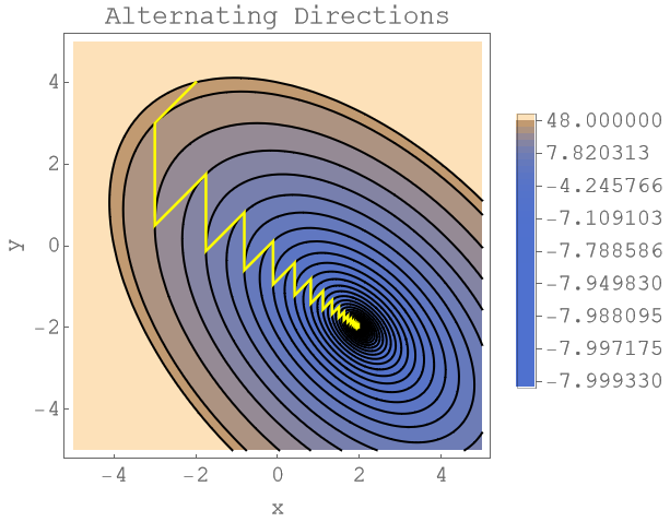
As we can see, there's a lot of wiggling around, especially towards the end. This makes this approach of alternating directions rather slow. You need a lot of iterations.

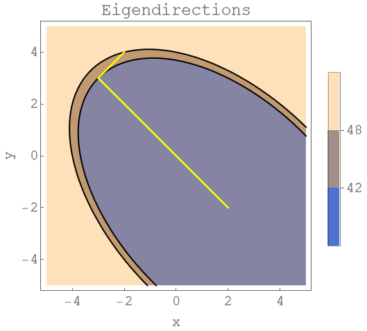
Note that if you chose the eigenvectors as directions, then you get to the solution rather quickly. In the plot below, two iterations are enough. Unfortunately computing the eigenvectors is usually more complicated and time consuming than solving the linear system directly. Unless we find a cheap and easy way to get the eigenvectors, this strategy is not really viable.

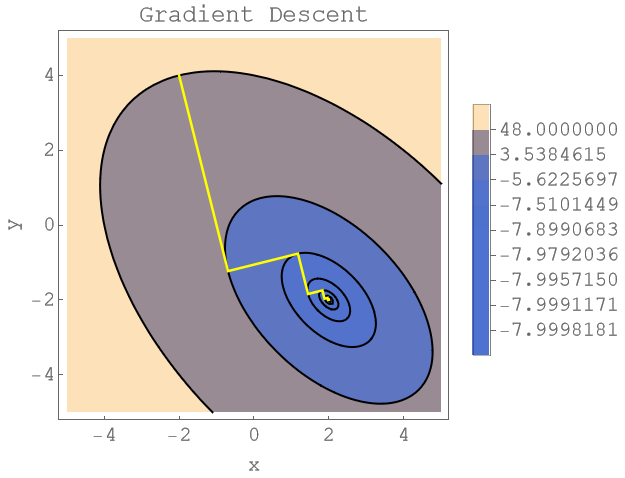
As mentionned above, the negative gradient points in the direction of the steepest descent. As we can see from the next plot, this leads to a faster convergence than the fixed arbitrary directions but it's actually slower than using the eigenvector directions. Also here, there's a lot of wiggling around the end. Nevertheless, gradient descent is a very popular approach which works quite well in many cases.

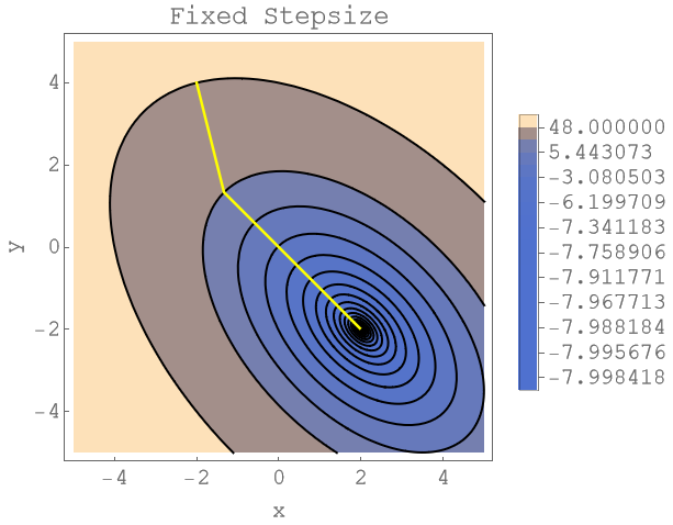
Finally, let's have a look what happens when you do not use the optimal step size. The next plot uses the gradient to descent direction but keeps the step size fixed at the inverse of the largest eigenvalue of $A$. We do need a lot more steps to get to the solution (each level line represents an iterate) as in the gradient descent strategy with optimized step sizes. Note that this strategy is mentionned in Stiefels paper as "Gesamtschrittverfahren" ([2], page 19)

From direction to (sub-)spaces

Next assume that we are still at some point $x_0$, but this time we want to minimize over the space spanned by the vectors $v_i$, $i=1$, ..., $n$. If we could minimize over more than one dimension at a time, we could significantly speed up our optimization strategy. Without loss of generality we can assume that all the $v_i$ are linearly independent. That means we want to solve

By a similar expansion as before we find the following equations

Which implies that the next residual vector will be orthogonal to all previous search directions if the $\lambda_i$ are chosen in an optimal way. Also, if $x_0$ is our sought solution, then the only possible choice for all $\lambda_i$ will be $\lambda_i=0$. Note that the optimal $\lambda_i$ must solve the following linear system of equations

This is a linear system of equations with a symmetric system matrix. The $(i,j)$-th entry of the system matrix is given by $\left\langle v_i, Av_j\right\rangle$. The unknowns are the $\lambda_i$ and the righthand side is given by $\left\langle Ax_0 - b, v_k\right\rangle$. Clearly this linear system of equations cannot have more equations than our initial system since we are optimizing over a subspace. Initially we required our system matrix to be positive definite. It would be interesting to know if this property carried over to this matrix. Positive definiteness of an arbitrary matrix $M$ means that for any non-zero vector $z$ we have $z^\top M z > 0$. In this case we end up with the expression

which will be 0 if and only if all $\lambda_i = 0$ because $A$ is positive definite and all $v_i$ are assumed to be linearly independent. Indeed, the only way for $\sum_j \lambda_j v_j$ to be 0 is by enforcing that all $\lambda_i$ are already 0.

The previous observation gives us another hint at how to minimize $E$. Rather than tackling the large linear system, we chose a certain subspace and derive a linear system with a smaller number of equations. Sometimes you encounter linear systems of equations where you know upfront that along certain directions nothing really interesting is going to happen. In such case you could deliberately ignore these directions from the beginning on.

Directional corrections

Stiefel presents another nice little trick in his paper that we will discuss in this section. He refers to it as "Pauschalkorrektur" ([2], page 22) and allows you to obtain an iterative scheme that finds the solution in a finite number of steps.

We begin with a simple definition. We say two vectors $u$ and $v$ are conjugate with respect to some symetric and positive definite matrix $A$ if $\langle u, Av\rangle = 0$. Obviously it follows that $\langle v, Au\rangle = 0$ holds then as well.

We mentioned above that the gradient is a convenient descent direction. Stiefel proposes in his paper the following slight adaptation. For the first descent direction we still use the negative gradient. For all subsequent iterates, rather than using the current negative gradient as descent direction, we consider

as update strategy. We add a correction to the descent direction that includes knowledge on previous descent directions. The scalar $\varepsilon_{k-1}$ shall be chosen such that $v_k$ will be $A$ conjugate to $v_{k-1}$. An easy computation reveals that this is the case if

Stiefel shows in his paper that the just mentionned update strategy generates a family of descent directions where each new direction will be $A$ conjugate to all previous directions. From this you can immediately conclude that you cannot generate more than $n$ iterates if you have a system with $n$ equations and unknowns.

If you assume that your solution $x$ can be expressed as $x=\sum_i\alpha_k v_k$, then a multiplication with $Av_j$ yields

From $Au-b=0$ it now follows by using the previous identity that

Which shows that we actually minimize over the spaces spanned by the vectors $v_j$!

The complete Algorithm

The full algorithm is now rather short and only consist of 4 steps. The iterative loop consists of

1. Computation of the "Pauschalkorrektur" $\varepsilon$.

2. Computation of the next descent direction $v$.

3. Computation of the corresponding step size $\lambda$.

4. Computation of the next residual.

Your entrypoint to the loop will be step 2 (with $\varepsilon=0$). You then iterate the previous 4 steps until you cannot find a new descent direction anymore. In the end, your solution is given by

where $x_0$ is some initial guess, $\lambda_j$ your step sizes and $v_j$ your search directions.

Source Code

The following Mathematica code implements the conjugate gradients method as presented in Stiefels paper [2] on page 26. Note that he solves $Ax+b=0$ rather than $Ax=b$. I have added the steps outlined in his paper as comments behind the corresponding lines.

CGStiefel[A_?MatrixQ, b_?VectorQ, x0_?VectorQ] := 
  Module[{solution, residual, stepSize, conjugateCorrection, 
    searchDirection, oldResidual},
   solution = x0;
   residual = A . x0 + b;
   searchDirection = -residual;(*2*)
   While[Dot[searchDirection, searchDirection] > 0,
    stepSize = 
     Dot[residual, residual]/
      Dot[A . searchDirection, searchDirection];(*3*)
    solution = solution + stepSize*searchDirection;
    oldResidual = residual;
    Assert[
     Dot[residual + stepSize*A . searchDirection, residual] == 0];
    residual = residual + stepSize*A . searchDirection;(*4*)
    conjugateCorrection = 
     Dot[residual, residual]/Dot[oldResidual, oldResidual];(*1*)
    Assert[
     Dot[-residual + conjugateCorrection*searchDirection, 
       A . searchDirection] == 0];
    searchDirection = -residual + 
      conjugateCorrection*searchDirection;(*2*)
    ];
   Return[{solution, A . solution + b}];
   ];

What does it have to do with Krylov subspaces?

The relationship to the Krylow subspaces is not really apparent here. As mentionned above, we minimise over the subspaces that are spanned by the descent directions $v$. One can show (c.f. [1]) that in each step, this subspace can also be described as

Here $x_0$ is your initial guess and $r_0$ is the corresponding residual. This shows that you are actually minimising over Krylov subspaces!

References

[1] A. Meister, Numerik linearer Gleichungssysteme, 5 ed. Springer Fachmedien Wiesbaden, 2015, p. 276. doi: 10.1007/978-3-658-07200-1.

[2] E. Stiefel, “Über einige Methoden der Relaxationsrechnung,” ZAMP Zeitschrift für angewandte Mathematik und Physik, vol. 3, no. 1, Art. no. 1, 1952-01, doi: 10.1007/bf02080981.

[3] R. Fletcher and C. M. Reeves, “Function minimization by conjugate gradients,” The Computer Journal, vol. 7, no. 2, Art. no. 2, 1964-02, doi: 10.1093/comjnl/7.2.149.

[4] E. Polak and G. Ribière, “Note sur la convergence de méthodes de directions conjuguées,” Rev. Française Informat Recherche Opérationelle, vol. 3, no. 1, Art. no. 1, 1969.

[5] M. R. Hestenes and E. L. Stiefel, “Methods of Conjugate Gradients for Solving Linear Systems,” Journal of Research of the National Bureau of Standards, vol. 49, no. 6, Art. no. 6, 1952-12, doi: 10.6028/jres.049.044.

Notes

The previous presentation started with a linear system and derived a suitable energy. In return this lead to some further restrictions for the choice of the system matrix. Tweaking the energy to allow other types of matrices is a very fascinating topic.

@online{conjugate-gradients,
  author   = {Hoeltgen, Laurent},
  title    = {Conjugate Gradients},
  date     = {2021-10-31},
  language = english
  url      = {https://www.laurenthoeltgen.name/content/blog/
              conjugate-gradients}
}